ADP 17회 실기 문제#
풀이가 궁금하시다면 단톡방에서 문의주세요!!! 올 때 광고클릭
Attention
캐글에 업로드된 다른 분들 코드 보러가기
데이터셋 링크
문제오류, 코드오류 댓글로 피드백주세요
Attention
1번
데이터 설명 : 집과 관련된 여러 수치들과 집의 가격, log1p 정규화된 price 컬럼 예측 하기
데이터 출처 : https://www.kaggle.com/c/house-prices-advanced-regression-techniques/data?select=train.csv 일부 전처리
data Url : https://raw.githubusercontent.com/Datamanim/datarepo/main/adp/p3/problem1.csv
import pandas as pd

df = pd.read_csv('https://raw.githubusercontent.com/Datamanim/datarepo/main/adp/17/problem1.csv')
df.head()
| Id | LotArea | LotFrontage | YearBuilt | 1stFlrSF | 2ndFlrSF | YearRemodAdd | TotRmsAbvGrd | KitchenAbvGr | BedroomAbvGr | GarageCars | GarageArea | price | |
|---|---|---|---|---|---|---|---|---|---|---|---|---|---|
| 0 | 1 | 8450 | 65.0 | 2003 | 856 | 854 | 2003 | 8 | 1 | 3 | 2 | 548 | 12.247699 |
| 1 | 2 | 9600 | 80.0 | 1976 | 1262 | 0 | 1976 | 6 | 1 | 3 | 2 | 460 | 12.109016 |
| 2 | 3 | 11250 | 68.0 | 2001 | 920 | 866 | 2002 | 6 | 1 | 3 | 2 | 608 | 12.317171 |
| 3 | 4 | 9550 | 60.0 | 1915 | 961 | 756 | 1970 | 7 | 1 | 3 | 3 | 642 | 11.849405 |
| 4 | 5 | 14260 | 84.0 | 2000 | 1145 | 1053 | 2000 | 9 | 1 | 4 | 3 | 836 | 12.429220 |
1-1번
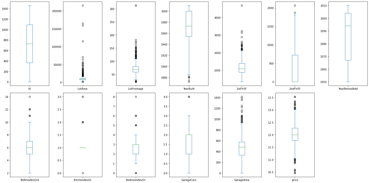
데이터 EDA 수행 후, 분석가 입장에서 의미있는 탐색
시각화 및 통계량 제시
Show code cell content
print(df.info())
display(df.describe())
print('''
모든 컬럼은 numeric 변수이다. 이상치가 존재하는 컬럼은 ~~ 이다. (중략)
''')

import matplotlib.pyplot as plt
df.plot(kind='box',subplots=True,layout=(2,len(df.columns)//2+1),figsize=(20,10))
plt.tight_layout()
plt.show()
<class 'pandas.core.frame.DataFrame'>
RangeIndex: 1460 entries, 0 to 1459
Data columns (total 13 columns):
 #   Column        Non-Null Count  Dtype
---  ------        --------------  -----
 0   Id            1460 non-null   int64
 1   LotArea       1460 non-null   int64
 2   LotFrontage   1201 non-null   float64
 3   YearBuilt     1460 non-null   int64
 4   1stFlrSF      1460 non-null   int64
 5   2ndFlrSF      1460 non-null   int64
 6   YearRemodAdd  1460 non-null   int64
 7   TotRmsAbvGrd  1460 non-null   int64
 8   KitchenAbvGr  1460 non-null   int64
 9   BedroomAbvGr  1460 non-null   int64
 10  GarageCars    1460 non-null   int64
 11  GarageArea    1460 non-null   int64
 12  price         1460 non-null   float64
dtypes: float64(2), int64(11)
memory usage: 148.4 KB
None
| Id | LotArea | LotFrontage | YearBuilt | 1stFlrSF | 2ndFlrSF | YearRemodAdd | TotRmsAbvGrd | KitchenAbvGr | BedroomAbvGr | GarageCars | GarageArea | price | |
|---|---|---|---|---|---|---|---|---|---|---|---|---|---|
| count | 1460.000000 | 1460.000000 | 1201.000000 | 1460.000000 | 1460.000000 | 1460.000000 | 1460.000000 | 1460.000000 | 1460.000000 | 1460.000000 | 1460.000000 | 1460.000000 | 1460.000000 |
| mean | 730.500000 | 10516.828082 | 70.049958 | 1971.267808 | 1162.626712 | 346.992466 | 1984.865753 | 6.517808 | 1.046575 | 2.866438 | 1.767123 | 472.980137 | 12.024057 |
| std | 421.610009 | 9981.264932 | 24.284752 | 30.202904 | 386.587738 | 436.528436 | 20.645407 | 1.625393 | 0.220338 | 0.815778 | 0.747315 | 213.804841 | 0.399449 |
| min | 1.000000 | 1300.000000 | 21.000000 | 1872.000000 | 334.000000 | 0.000000 | 1950.000000 | 2.000000 | 0.000000 | 0.000000 | 0.000000 | 0.000000 | 10.460271 |
| 25% | 365.750000 | 7553.500000 | 59.000000 | 1954.000000 | 882.000000 | 0.000000 | 1967.000000 | 5.000000 | 1.000000 | 2.000000 | 1.000000 | 334.500000 | 11.775105 |
| 50% | 730.500000 | 9478.500000 | 69.000000 | 1973.000000 | 1087.000000 | 0.000000 | 1994.000000 | 6.000000 | 1.000000 | 3.000000 | 2.000000 | 480.000000 | 12.001512 |
| 75% | 1095.250000 | 11601.500000 | 80.000000 | 2000.000000 | 1391.250000 | 728.000000 | 2004.000000 | 7.000000 | 1.000000 | 3.000000 | 2.000000 | 576.000000 | 12.273736 |
| max | 1460.000000 | 215245.000000 | 313.000000 | 2010.000000 | 4692.000000 | 2065.000000 | 2010.000000 | 14.000000 | 3.000000 | 8.000000 | 4.000000 | 1418.000000 | 13.534474 |
모든 컬럼은 numeric 변수이다. 이상치가 존재하는 컬럼은 ~~ 이다. (중략)
1-2번
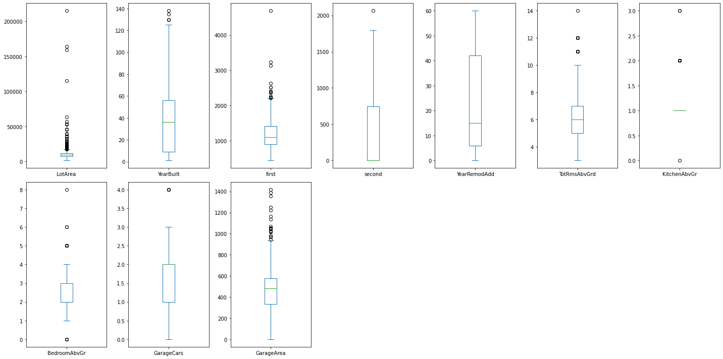
Train,Valid,Test set으로 분할 및 시각화 제시
Show code cell content
df2 = df.copy()

#컬럼에 숫자가 들어가면 statsmodels ols 동작시 에러발생
df2 = df2.rename(columns={'1stFlrSF':'first','2ndFlrSF':'second'})

#년도 데이터의 경우 최대년도 기준 몇년전인지 값으로 대체
df2['YearBuilt']  = abs(df2['YearBuilt'] - df2['YearBuilt'].max())
df2['YearRemodAdd']  = abs(df2['YearRemodAdd'] - df2['YearRemodAdd'].max())


X = df2.drop(columns=['Id','price','LotFrontage'])
y = df2['price']

from sklearn.model_selection import train_test_split
from sklearn.preprocessing import StandardScaler

X_train, X_test , y_train, y_test = train_test_split(X,y)

sc = StandardScaler()
sc.fit(X_train)

X_train_sc = sc.transform(X_train)
X_test_sc = sc.transform(X_test)

print('스케일링 전 시각화')
X_train.plot(kind='box',subplots=True,layout=(2,len(df.columns)//2+1),figsize=(20,10))
plt.tight_layout()
plt.show()
print('스케일링 후 시각화')
pd.DataFrame(X_train_sc,columns=X_train.columns).plot(kind='box',subplots=True,layout=(2,len(df.columns)//2+1),figsize=(20,10))
plt.tight_layout()
plt.show()


print('''
설명 ~~(생략)) -> 회귀 분석시 스케일링 하지 않는 것이 r-squred 값이 더 높게나옴
''')
스케일링 전 시각화
스케일링 후 시각화
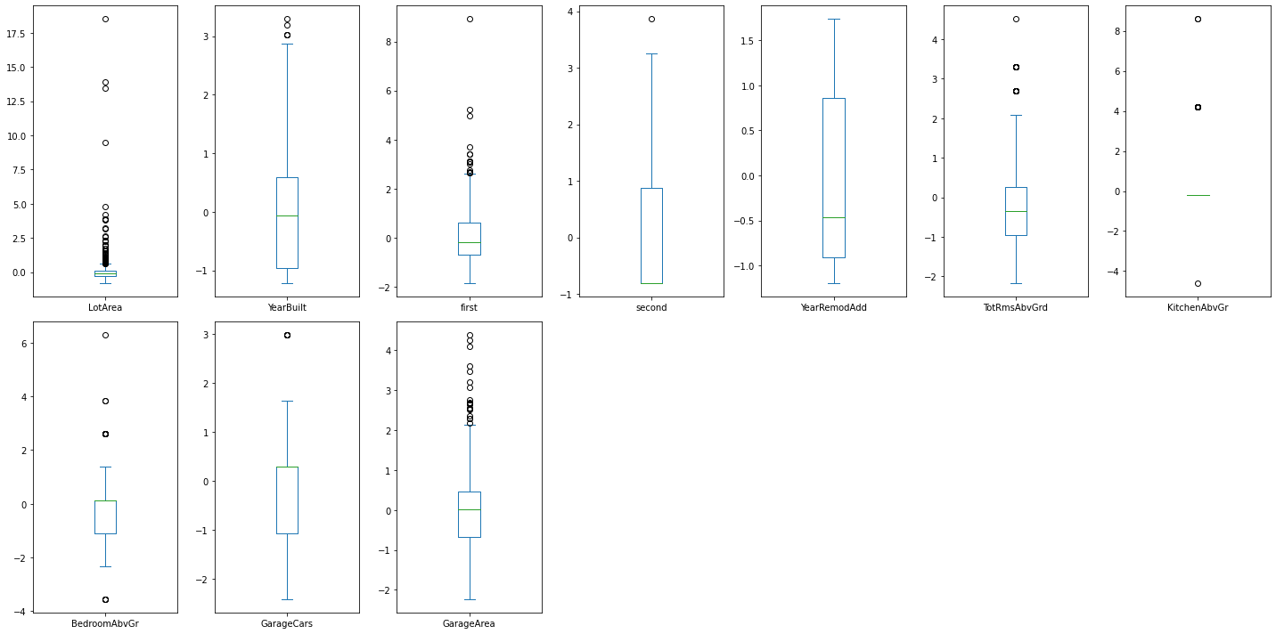
설명 ~~(생략)) -> 회귀 분석시 스케일링 하지 않는 것이 r-squred 값이 더 높게나옴
1-3번
2차 교호작용항 까지 고려한 회귀분석 수행 및 변수 선택 과정 제시
Show code cell content
from itertools import permutations
comb = list(permutations(X_train.columns, 3))
len(comb)

variables= '+ '.join(list(X_train.columns)) +'+'+ '+'.join([':'.join(list(y)) for y in comb])
# 파이썬은 회귀분석에 있어 모듈이 불친철 한거같네요 ㅎㅎ ㅠ
# 아래의 2차 교호 작용을 모두 포함한 컬럼중에서 각자의 기준에 맞게 변수 선택하시며 될 것 같습니다.
# 모든 변수 포함시 단순 다항회귀보다는 r-squared값이 높게 나옵니다

from statsmodels.formula.api import ols

#'+ '.join(list(X_train.columns))
res = ols(f'price ~ {variables}', data=pd.concat([X_train,y_train],axis=1)).fit()
res.summary()
| Dep. Variable: | price | R-squared: | 0.882 |
|---|---|---|---|
| Model: | OLS | Adj. R-squared: | 0.866 |
| Method: | Least Squares | F-statistic: | 55.46 |
| Date: | Sun, 04 Sep 2022 | Prob (F-statistic): | 0.00 |
| Time: | 19:43:15 | Log-Likelihood: | 627.85 |
| No. Observations: | 1095 | AIC: | -993.7 |
| Df Residuals: | 964 | BIC: | -338.9 |
| Df Model: | 130 | ||
| Covariance Type: | nonrobust |
| coef | std err | t | P>|t| | [0.025 | 0.975] | |
|---|---|---|---|---|---|---|
| Intercept | 11.0885 | 0.138 | 80.418 | 0.000 | 10.818 | 11.359 |
| LotArea | 1.681e-05 | 6.03e-06 | 2.789 | 0.005 | 4.98e-06 | 2.86e-05 |
| YearBuilt | -0.0028 | 0.001 | -3.388 | 0.001 | -0.004 | -0.001 |
| first | 0.0008 | 0.000 | 6.271 | 0.000 | 0.001 | 0.001 |
| second | 0.0004 | 0.000 | 3.386 | 0.001 | 0.000 | 0.001 |
| YearRemodAdd | -0.0007 | 0.001 | -0.507 | 0.612 | -0.003 | 0.002 |
| TotRmsAbvGrd | 0.0192 | 0.027 | 0.717 | 0.474 | -0.033 | 0.072 |
| KitchenAbvGr | -0.1496 | 0.110 | -1.355 | 0.176 | -0.366 | 0.067 |
| BedroomAbvGr | -0.0182 | 0.032 | -0.571 | 0.568 | -0.081 | 0.044 |
| GarageCars | -0.0502 | 0.070 | -0.717 | 0.473 | -0.188 | 0.087 |
| GarageArea | 0.0005 | 0.000 | 2.074 | 0.038 | 2.94e-05 | 0.001 |
| LotArea:YearBuilt:first | -1.855e-10 | 2.29e-10 | -0.809 | 0.419 | -6.36e-10 | 2.65e-10 |
| LotArea:YearBuilt:second | 7.074e-10 | 2.41e-10 | 2.938 | 0.003 | 2.35e-10 | 1.18e-09 |
| LotArea:YearBuilt:YearRemodAdd | -1.303e-09 | 2.99e-09 | -0.435 | 0.664 | -7.18e-09 | 4.57e-09 |
| LotArea:YearBuilt:TotRmsAbvGrd | 3.239e-08 | 6.39e-08 | 0.507 | 0.612 | -9.3e-08 | 1.58e-07 |
| LotArea:YearBuilt:KitchenAbvGr | 2.606e-07 | 2.36e-07 | 1.104 | 0.270 | -2.03e-07 | 7.24e-07 |
| LotArea:YearBuilt:BedroomAbvGr | -2.779e-07 | 1.13e-07 | -2.469 | 0.014 | -4.99e-07 | -5.7e-08 |
| LotArea:YearBuilt:GarageCars | 6.293e-09 | 1.82e-07 | 0.035 | 0.972 | -3.51e-07 | 3.64e-07 |
| LotArea:YearBuilt:GarageArea | 6.611e-10 | 5.9e-10 | 1.121 | 0.263 | -4.97e-10 | 1.82e-09 |
| LotArea:first:second | -4.53e-11 | 1e-11 | -4.516 | 0.000 | -6.5e-11 | -2.56e-11 |
| LotArea:first:YearRemodAdd | -6.024e-10 | 2.96e-10 | -2.037 | 0.042 | -1.18e-09 | -2.22e-11 |
| LotArea:first:TotRmsAbvGrd | -6.169e-10 | 1.68e-09 | -0.367 | 0.713 | -3.91e-09 | 2.68e-09 |
| LotArea:first:KitchenAbvGr | -2.641e-08 | 2.05e-08 | -1.285 | 0.199 | -6.67e-08 | 1.39e-08 |
| LotArea:first:BedroomAbvGr | 1.835e-08 | 6.38e-09 | 2.875 | 0.004 | 5.82e-09 | 3.09e-08 |
| LotArea:first:GarageCars | 5.49e-09 | 8.44e-09 | 0.650 | 0.516 | -1.11e-08 | 2.21e-08 |
| LotArea:first:GarageArea | -1.098e-11 | 1.72e-11 | -0.640 | 0.523 | -4.47e-11 | 2.27e-11 |
| LotArea:second:YearRemodAdd | -8.782e-10 | 3.1e-10 | -2.832 | 0.005 | -1.49e-09 | -2.7e-10 |
| LotArea:second:TotRmsAbvGrd | 2.032e-09 | 2.62e-09 | 0.775 | 0.439 | -3.11e-09 | 7.18e-09 |
| LotArea:second:KitchenAbvGr | -3.869e-08 | 2.59e-08 | -1.493 | 0.136 | -8.95e-08 | 1.22e-08 |
| LotArea:second:BedroomAbvGr | 2.198e-08 | 6.62e-09 | 3.318 | 0.001 | 8.98e-09 | 3.5e-08 |
| LotArea:second:GarageCars | 1.307e-08 | 1.57e-08 | 0.834 | 0.405 | -1.77e-08 | 4.38e-08 |
| LotArea:second:GarageArea | -3.094e-11 | 4.75e-11 | -0.652 | 0.515 | -1.24e-10 | 6.23e-11 |
| LotArea:YearRemodAdd:TotRmsAbvGrd | 5.427e-09 | 8.01e-08 | 0.068 | 0.946 | -1.52e-07 | 1.63e-07 |
| LotArea:YearRemodAdd:KitchenAbvGr | -4.554e-07 | 3.4e-07 | -1.341 | 0.180 | -1.12e-06 | 2.11e-07 |
| LotArea:YearRemodAdd:BedroomAbvGr | 3.882e-07 | 1.36e-07 | 2.844 | 0.005 | 1.2e-07 | 6.56e-07 |
| LotArea:YearRemodAdd:GarageCars | 4.172e-07 | 2.4e-07 | 1.735 | 0.083 | -5.47e-08 | 8.89e-07 |
| LotArea:YearRemodAdd:GarageArea | -9.078e-10 | 8.25e-10 | -1.101 | 0.271 | -2.53e-09 | 7.11e-10 |
| LotArea:TotRmsAbvGrd:KitchenAbvGr | 5.611e-06 | 5.75e-06 | 0.976 | 0.329 | -5.67e-06 | 1.69e-05 |
| LotArea:TotRmsAbvGrd:BedroomAbvGr | -3.3e-06 | 1.66e-06 | -1.990 | 0.047 | -6.56e-06 | -4.51e-08 |
| LotArea:TotRmsAbvGrd:GarageCars | 1.408e-06 | 4.66e-06 | 0.302 | 0.762 | -7.73e-06 | 1.05e-05 |
| LotArea:TotRmsAbvGrd:GarageArea | -1.493e-10 | 1.22e-08 | -0.012 | 0.990 | -2.4e-08 | 2.37e-08 |
| LotArea:KitchenAbvGr:BedroomAbvGr | 5.376e-06 | 8.57e-06 | 0.628 | 0.530 | -1.14e-05 | 2.22e-05 |
| LotArea:KitchenAbvGr:GarageCars | 2.764e-05 | 1.78e-05 | 1.554 | 0.120 | -7.26e-06 | 6.25e-05 |
| LotArea:KitchenAbvGr:GarageArea | -1.531e-07 | 6.26e-08 | -2.446 | 0.015 | -2.76e-07 | -3.02e-08 |
| LotArea:BedroomAbvGr:GarageCars | -1.998e-05 | 6.02e-06 | -3.320 | 0.001 | -3.18e-05 | -8.17e-06 |
| LotArea:BedroomAbvGr:GarageArea | 5.249e-08 | 1.91e-08 | 2.746 | 0.006 | 1.5e-08 | 9e-08 |
| LotArea:GarageCars:GarageArea | 8.292e-09 | 6.46e-09 | 1.283 | 0.200 | -4.39e-09 | 2.1e-08 |
| YearBuilt:first:second | 6.499e-09 | 2.89e-09 | 2.251 | 0.025 | 8.33e-10 | 1.22e-08 |
| YearBuilt:first:YearRemodAdd | -9.716e-09 | 5.52e-08 | -0.176 | 0.860 | -1.18e-07 | 9.87e-08 |
| YearBuilt:first:TotRmsAbvGrd | -6.298e-07 | 6.83e-07 | -0.922 | 0.357 | -1.97e-06 | 7.11e-07 |
| YearBuilt:first:KitchenAbvGr | 7.531e-06 | 3.58e-06 | 2.102 | 0.036 | 5e-07 | 1.46e-05 |
| YearBuilt:first:BedroomAbvGr | -1.598e-06 | 1.41e-06 | -1.137 | 0.256 | -4.36e-06 | 1.16e-06 |
| YearBuilt:first:GarageCars | -1.138e-06 | 2.55e-06 | -0.446 | 0.656 | -6.14e-06 | 3.87e-06 |
| YearBuilt:first:GarageArea | -3.338e-10 | 8.6e-09 | -0.039 | 0.969 | -1.72e-08 | 1.65e-08 |
| YearBuilt:second:YearRemodAdd | -2.12e-08 | 4.98e-08 | -0.426 | 0.670 | -1.19e-07 | 7.65e-08 |
| YearBuilt:second:TotRmsAbvGrd | -6.959e-07 | 6.56e-07 | -1.061 | 0.289 | -1.98e-06 | 5.92e-07 |
| YearBuilt:second:KitchenAbvGr | -9.564e-08 | 3.24e-06 | -0.030 | 0.976 | -6.45e-06 | 6.25e-06 |
| YearBuilt:second:BedroomAbvGr | -1.143e-06 | 1.24e-06 | -0.921 | 0.357 | -3.58e-06 | 1.29e-06 |
| YearBuilt:second:GarageCars | 6.176e-07 | 2.02e-06 | 0.306 | 0.760 | -3.34e-06 | 4.58e-06 |
| YearBuilt:second:GarageArea | -1.089e-08 | 7.51e-09 | -1.450 | 0.147 | -2.56e-08 | 3.85e-09 |
| YearBuilt:YearRemodAdd:TotRmsAbvGrd | 1.153e-05 | 1.31e-05 | 0.882 | 0.378 | -1.41e-05 | 3.72e-05 |
| YearBuilt:YearRemodAdd:KitchenAbvGr | -7.995e-05 | 3.49e-05 | -2.289 | 0.022 | -0.000 | -1.14e-05 |
| YearBuilt:YearRemodAdd:BedroomAbvGr | 6.674e-06 | 1.97e-05 | 0.339 | 0.735 | -3.19e-05 | 4.53e-05 |
| YearBuilt:YearRemodAdd:GarageCars | -9.502e-07 | 3.21e-05 | -0.030 | 0.976 | -6.4e-05 | 6.21e-05 |
| YearBuilt:YearRemodAdd:GarageArea | -4.09e-09 | 1.22e-07 | -0.033 | 0.973 | -2.44e-07 | 2.36e-07 |
| YearBuilt:TotRmsAbvGrd:KitchenAbvGr | -0.0008 | 0.001 | -1.265 | 0.206 | -0.002 | 0.000 |
| YearBuilt:TotRmsAbvGrd:BedroomAbvGr | 0.0005 | 0.000 | 2.521 | 0.012 | 0.000 | 0.001 |
| YearBuilt:TotRmsAbvGrd:GarageCars | -8.21e-05 | 0.001 | -0.108 | 0.914 | -0.002 | 0.001 |
| YearBuilt:TotRmsAbvGrd:GarageArea | -5.181e-07 | 2.65e-06 | -0.196 | 0.845 | -5.72e-06 | 4.68e-06 |
| YearBuilt:KitchenAbvGr:BedroomAbvGr | -0.0006 | 0.001 | -0.493 | 0.622 | -0.003 | 0.002 |
| YearBuilt:KitchenAbvGr:GarageCars | -0.0016 | 0.003 | -0.611 | 0.541 | -0.007 | 0.003 |
| YearBuilt:KitchenAbvGr:GarageArea | 4.112e-06 | 9.28e-06 | 0.443 | 0.658 | -1.41e-05 | 2.23e-05 |
| YearBuilt:BedroomAbvGr:GarageCars | 0.0014 | 0.001 | 1.153 | 0.249 | -0.001 | 0.004 |
| YearBuilt:BedroomAbvGr:GarageArea | 6.209e-07 | 4.55e-06 | 0.137 | 0.891 | -8.3e-06 | 9.54e-06 |
| YearBuilt:GarageCars:GarageArea | -2.734e-06 | 1.46e-06 | -1.877 | 0.061 | -5.59e-06 | 1.25e-07 |
| first:second:YearRemodAdd | 8.914e-09 | 4.59e-09 | 1.944 | 0.052 | -8.63e-11 | 1.79e-08 |
| first:second:TotRmsAbvGrd | 4.955e-08 | 4.02e-08 | 1.233 | 0.218 | -2.93e-08 | 1.28e-07 |
| first:second:KitchenAbvGr | -9.975e-07 | 2.77e-07 | -3.602 | 0.000 | -1.54e-06 | -4.54e-07 |
| first:second:BedroomAbvGr | 2.191e-08 | 8.32e-08 | 0.263 | 0.792 | -1.41e-07 | 1.85e-07 |
| first:second:GarageCars | 3.508e-08 | 2.05e-07 | 0.171 | 0.864 | -3.68e-07 | 4.38e-07 |
| first:second:GarageArea | 1.031e-09 | 6.88e-10 | 1.498 | 0.134 | -3.2e-10 | 2.38e-09 |
| first:YearRemodAdd:TotRmsAbvGrd | 6.648e-07 | 1.09e-06 | 0.609 | 0.543 | -1.48e-06 | 2.81e-06 |
| first:YearRemodAdd:KitchenAbvGr | 2.789e-07 | 6.16e-06 | 0.045 | 0.964 | -1.18e-05 | 1.24e-05 |
| first:YearRemodAdd:BedroomAbvGr | -4.57e-07 | 2.09e-06 | -0.219 | 0.827 | -4.56e-06 | 3.64e-06 |
| first:YearRemodAdd:GarageCars | 1.289e-06 | 4.63e-06 | 0.278 | 0.781 | -7.8e-06 | 1.04e-05 |
| first:YearRemodAdd:GarageArea | -6.344e-09 | 1.52e-08 | -0.417 | 0.677 | -3.62e-08 | 2.35e-08 |
| first:TotRmsAbvGrd:KitchenAbvGr | -3.896e-05 | 3.88e-05 | -1.003 | 0.316 | -0.000 | 3.73e-05 |
| first:TotRmsAbvGrd:BedroomAbvGr | -7.693e-06 | 9.64e-06 | -0.798 | 0.425 | -2.66e-05 | 1.12e-05 |
| first:TotRmsAbvGrd:GarageCars | -3.116e-05 | 3.42e-05 | -0.911 | 0.363 | -9.83e-05 | 3.6e-05 |
| first:TotRmsAbvGrd:GarageArea | 1.945e-07 | 1.16e-07 | 1.675 | 0.094 | -3.34e-08 | 4.22e-07 |
| first:KitchenAbvGr:BedroomAbvGr | 4.232e-05 | 0.000 | 0.387 | 0.699 | -0.000 | 0.000 |
| first:KitchenAbvGr:GarageCars | 0.0002 | 0.000 | 0.607 | 0.544 | -0.000 | 0.001 |
| first:KitchenAbvGr:GarageArea | 3.252e-07 | 1.04e-06 | 0.312 | 0.755 | -1.72e-06 | 2.37e-06 |
| first:BedroomAbvGr:GarageCars | 6.764e-05 | 9.75e-05 | 0.694 | 0.488 | -0.000 | 0.000 |
| first:BedroomAbvGr:GarageArea | -5.945e-07 | 3.32e-07 | -1.789 | 0.074 | -1.25e-06 | 5.76e-08 |
| first:GarageCars:GarageArea | -2.502e-07 | 1.38e-07 | -1.807 | 0.071 | -5.22e-07 | 2.16e-08 |
| second:YearRemodAdd:TotRmsAbvGrd | -5.583e-07 | 1.08e-06 | -0.517 | 0.605 | -2.68e-06 | 1.56e-06 |
| second:YearRemodAdd:KitchenAbvGr | 1.737e-06 | 5.14e-06 | 0.338 | 0.735 | -8.34e-06 | 1.18e-05 |
| second:YearRemodAdd:BedroomAbvGr | -1.305e-06 | 1.9e-06 | -0.689 | 0.491 | -5.02e-06 | 2.41e-06 |
| second:YearRemodAdd:GarageCars | 7.759e-07 | 4.03e-06 | 0.193 | 0.847 | -7.13e-06 | 8.68e-06 |
| second:YearRemodAdd:GarageArea | 1.743e-09 | 1.4e-08 | 0.125 | 0.901 | -2.57e-08 | 2.91e-08 |
| second:TotRmsAbvGrd:KitchenAbvGr | 0.0001 | 5.23e-05 | 2.808 | 0.005 | 4.42e-05 | 0.000 |
| second:TotRmsAbvGrd:BedroomAbvGr | -1.089e-05 | 1.01e-05 | -1.073 | 0.284 | -3.08e-05 | 9.02e-06 |
| second:TotRmsAbvGrd:GarageCars | -4.411e-05 | 4.88e-05 | -0.904 | 0.366 | -0.000 | 5.17e-05 |
| second:TotRmsAbvGrd:GarageArea | -1.11e-07 | 1.69e-07 | -0.657 | 0.511 | -4.42e-07 | 2.2e-07 |
| second:KitchenAbvGr:BedroomAbvGr | -4.021e-05 | 0.000 | -0.389 | 0.697 | -0.000 | 0.000 |
| second:KitchenAbvGr:GarageCars | 0.0001 | 0.000 | 0.448 | 0.655 | -0.000 | 0.001 |
| second:KitchenAbvGr:GarageArea | 7.039e-07 | 9.34e-07 | 0.754 | 0.451 | -1.13e-06 | 2.54e-06 |
| second:BedroomAbvGr:GarageCars | 4.966e-06 | 8.41e-05 | 0.059 | 0.953 | -0.000 | 0.000 |
| second:BedroomAbvGr:GarageArea | -1.945e-07 | 2.83e-07 | -0.686 | 0.493 | -7.5e-07 | 3.62e-07 |
| second:GarageCars:GarageArea | 4.72e-09 | 1.49e-07 | 0.032 | 0.975 | -2.87e-07 | 2.96e-07 |
| YearRemodAdd:TotRmsAbvGrd:KitchenAbvGr | 0.0002 | 0.001 | 0.215 | 0.830 | -0.002 | 0.002 |
| YearRemodAdd:TotRmsAbvGrd:BedroomAbvGr | -0.0004 | 0.000 | -1.091 | 0.276 | -0.001 | 0.000 |
| YearRemodAdd:TotRmsAbvGrd:GarageCars | -0.0002 | 0.001 | -0.186 | 0.852 | -0.003 | 0.002 |
| YearRemodAdd:TotRmsAbvGrd:GarageArea | 2.171e-06 | 4.68e-06 | 0.463 | 0.643 | -7.02e-06 | 1.14e-05 |
| YearRemodAdd:KitchenAbvGr:BedroomAbvGr | 0.0011 | 0.002 | 0.623 | 0.534 | -0.002 | 0.004 |
| YearRemodAdd:KitchenAbvGr:GarageCars | -0.0033 | 0.004 | -0.807 | 0.420 | -0.011 | 0.005 |
| YearRemodAdd:KitchenAbvGr:GarageArea | 1.832e-05 | 1.5e-05 | 1.218 | 0.223 | -1.12e-05 | 4.78e-05 |
| YearRemodAdd:BedroomAbvGr:GarageCars | 0.0009 | 0.002 | 0.489 | 0.625 | -0.003 | 0.004 |
| YearRemodAdd:BedroomAbvGr:GarageArea | -5.439e-06 | 6.77e-06 | -0.803 | 0.422 | -1.87e-05 | 7.85e-06 |
| YearRemodAdd:GarageCars:GarageArea | -5.993e-06 | 2.44e-06 | -2.461 | 0.014 | -1.08e-05 | -1.21e-06 |
| TotRmsAbvGrd:KitchenAbvGr:BedroomAbvGr | -0.0005 | 0.017 | -0.029 | 0.977 | -0.033 | 0.032 |
| TotRmsAbvGrd:KitchenAbvGr:GarageCars | -0.0065 | 0.049 | -0.134 | 0.894 | -0.103 | 0.089 |
| TotRmsAbvGrd:KitchenAbvGr:GarageArea | -0.0001 | 0.000 | -0.506 | 0.613 | -0.001 | 0.000 |
| TotRmsAbvGrd:BedroomAbvGr:GarageCars | 0.0196 | 0.021 | 0.930 | 0.353 | -0.022 | 0.061 |
| TotRmsAbvGrd:BedroomAbvGr:GarageArea | -3.336e-06 | 7.56e-05 | -0.044 | 0.965 | -0.000 | 0.000 |
| TotRmsAbvGrd:GarageCars:GarageArea | -2.25e-05 | 4.05e-05 | -0.556 | 0.578 | -0.000 | 5.69e-05 |
| KitchenAbvGr:BedroomAbvGr:GarageCars | -0.1129 | 0.088 | -1.280 | 0.201 | -0.286 | 0.060 |
| KitchenAbvGr:BedroomAbvGr:GarageArea | 0.0002 | 0.000 | 0.532 | 0.595 | -0.000 | 0.001 |
| KitchenAbvGr:GarageCars:GarageArea | 0.0002 | 0.000 | 1.323 | 0.186 | -8.19e-05 | 0.000 |
| BedroomAbvGr:GarageCars:GarageArea | 0.0001 | 6.05e-05 | 1.859 | 0.063 | -6.24e-06 | 0.000 |
| Omnibus: | 273.758 | Durbin-Watson: | 1.905 |
|---|---|---|---|
| Prob(Omnibus): | 0.000 | Jarque-Bera (JB): | 1531.811 |
| Skew: | -1.030 | Prob(JB): | 0.00 |
| Kurtosis: | 8.416 | Cond. No. | 8.86e+11 |
Notes:
[1] Standard Errors assume that the covariance matrix of the errors is correctly specified.
[2] The condition number is large, 8.86e+11. This might indicate that there are
strong multicollinearity or other numerical problems.
1-4번
벌점, 앙상블을 포함하여 모형에 적합한 기계학습 모델 3가지를 제시하라
(평가지표는 MSE, MAPE, R2 모두 확인할 것)
Show code cell content
# lasso , ridge , randomforest
import numpy as np
from sklearn.linear_model import Lasso
from sklearn.linear_model import Ridge
from sklearn.ensemble import RandomForestRegressor
from sklearn.metrics import mean_squared_error , r2_score
def MAPE(y_test, y_pred):
    return np.mean(np.abs((y_test - y_pred) / y_test)) * 100


ls = Lasso()
rd = Ridge()
rf = RandomForestRegressor()


def modelpipe(model):

    model.fit(X_train,y_train)
    model_pred = model.predict(X_test)
    mse = mean_squared_error(y_test,model_pred)
    r2score = r2_score(y_test,model_pred)
    mape = MAPE(y_test,model_pred)

    metrics= [mse,r2score,mape]
    return metrics

ls_result =modelpipe(ls)
rd_result =modelpipe(rd)
rf_result =modelpipe(rf)


result = pd.DataFrame([ls_result,rd_result,rf_result],columns = ['mse','r2','mape'],index=['lasso','ridge','randomForest'])
result
| mse | r2 | mape | |
|---|---|---|---|
| lasso | 0.036525 | 0.773635 | 1.112493 |
| ridge | 0.032585 | 0.798051 | 1.067809 |
| randomForest | 0.034023 | 0.789136 | 1.071550 |
Attention
2번
데이터 설명 : 코로나19에 대한 나라별 데이터로 모델링 진행
데이터 출처 : https://www.kaggle.com/imdevskp/corona-virus-report 일부 후처리
data Url : https://raw.githubusercontent.com/Datamanim/datarepo/main/adp/p3/problem2.csv
location : 지역명
date : 일자
total_cases : 누적 확인자
total_deaths : 누적 사망자
new_tests : 검사자
population : 인구
new_vaccinations : 백신 접종자
import pandas as pd
df =pd.read_csv('https://raw.githubusercontent.com/Datamanim/datarepo/main/adp/17/problem2.csv')
df.head()
| location | date | total_cases | total_deaths | new_tests | population | new_vaccinations | |
|---|---|---|---|---|---|---|---|
| 0 | Afghanistan | 2020-02-24 | 5.0 | NaN | NaN | 39835428.0 | NaN |
| 1 | Afghanistan | 2020-02-25 | 5.0 | NaN | NaN | 39835428.0 | NaN |
| 2 | Afghanistan | 2020-02-26 | 5.0 | NaN | NaN | 39835428.0 | NaN |
| 3 | Afghanistan | 2020-02-27 | 5.0 | NaN | NaN | 39835428.0 | NaN |
| 4 | Afghanistan | 2020-02-28 | 5.0 | NaN | NaN | 39835428.0 | NaN |
2-1번
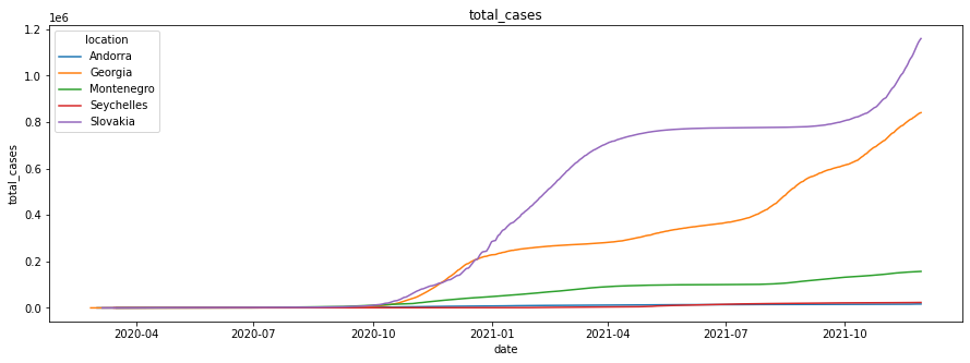
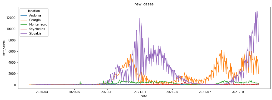
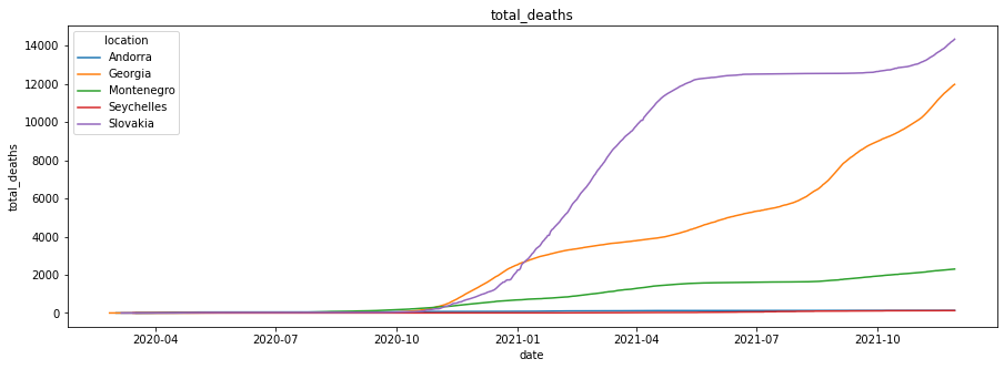
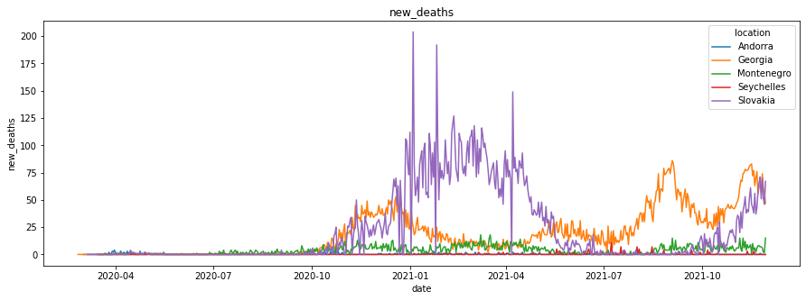
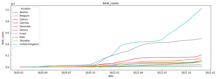
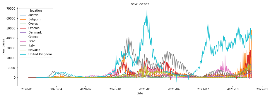
마지막 일자를 기준으로 인구 대비 확진자 비율이 높은 상위 5개 국가를 구하여라
상위 5개 국가별로 누적 확진자, 일일 확진자, 누적 사망자, 일일 사망자, 그래프, 범례를 이용해서 가독성 있게 만들어라
Show code cell content
df =pd.read_csv('https://raw.githubusercontent.com/Datamanim/datarepo/main/adp/17/problem2.csv')
df['ratio'] = df['total_cases'] / df['population']


# 전체 데이터의 결측치 및 일일 확진, 사망자 확인
# 2021-11-30에는 new_tests , new_vaccinations값이 nan 이므로 제외
# 인구수 0인 케이스 제외
import matplotlib.pyplot as plt
df = df.fillna(0)
df['date']  = pd.to_datetime(df['date'])
df = df[df.date != pd.to_datetime('2021-11-30')]
df = df[df.population !=0]

for location in df.location.unique():
    lo = df[df.location == location]
    df.loc[lo.index,'new_cases'] =lo.total_cases.diff().values
    df.loc[lo.index[0], 'new_cases'] = lo['total_cases'].values[0]

    df.loc[lo.index,'new_deaths'] =lo.total_deaths.diff().values
    df.loc[lo.index[0], 'new_deaths'] = lo['total_deaths'].values[0]

    df.loc[lo.index, 'total_vacciantions'] = lo['new_vaccinations'].cumsum().values
    df.loc[lo.index, '7days_new_case'] = lo['new_tests'].rolling(7).sum().fillna(0).values

import seaborn as sns
import matplotlib.pyplot as plt


locations = df.groupby(['location']).tail(1).sort_values('ratio',ascending=False).location.head(5).values
target = df[df.location.isin(locations)].reset_index(drop=True)
for v in ['total_cases','new_cases','total_deaths','new_deaths']:
    plt.figure(figsize = (15,5))
    plt.title(v)
    sns.lineplot(data=target,x= 'date',y=v,hue='location')
    plt.show()
2-2번
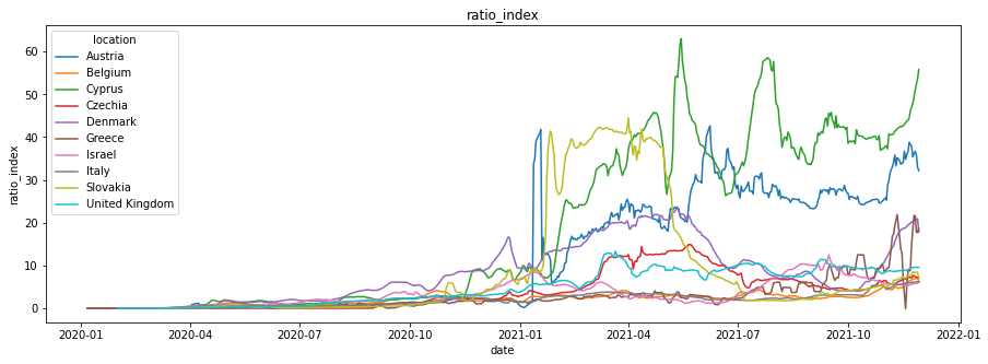
코로나 위험지수를 직접 만들고 그 위험지수에 대한 설명을 적고 위험지수가 높은 국가들 10개를 선정해서 시각화
Show code cell content
# 위험지수 =  ( 최근일주일 누적 확진자 / 인구수)   + (일일 사망자 / 인구수) - (누적 백신 인구 / 인구수) * 보정 상수) * 보정 상수
print('''
코로나 위험지수는 코로나로 인한 국가의 위기정도를 표현한다. 코로나 전파 특성상 최근 일주일의 확진자 숫자가 그다음의 일주일에 영향을 준다.
일일 사망자수는 현재 코로나의 국가 내에서의 치명율을 표현한다. 위기정도는 누적 백신인구에 의해 감소 될수 있다.
국가간의 비교를 위해 각 국가의 인구수로 나눠주어 값을 스케일링하고, 변수간 보정상수를 통해 정수화를 유도한다
''')

def ratio_index(x):
    value = (x['7days_new_case'] / x['population'] + x['new_deaths'] / x['population'] - x['total_vacciantions'] / x['population']*0.001) *100
    return value


df['ratio_index'] = df.apply(ratio_index,axis=1)


locations = df.groupby(['location']).tail(1).sort_values('ratio_index',ascending=False).location.head(10).values
target = df[df.location.isin(locations)].reset_index(drop=True)
for v in ['total_cases','new_cases','ratio_index']:
    plt.figure(figsize = (15,5))
    plt.title(v)
    sns.lineplot(data=target,x= 'date',y=v,hue='location')
    plt.show()
코로나 위험지수는 코로나로 인한 국가의 위기정도를 표현한다. 코로나 전파 특성상 최근 일주일의 확진자 숫자가 그다음의 일주일에 영향을 준다.
일일 사망자수는 현재 코로나의 국가 내에서의 치명율을 표현한다. 위기정도는 누적 백신인구에 의해 감소 될수 있다.
국가간의 비교를 위해 각 국가의 인구수로 나눠주어 값을 스케일링하고, 변수간 보정상수를 통해 정수화를 유도한다
2-3번
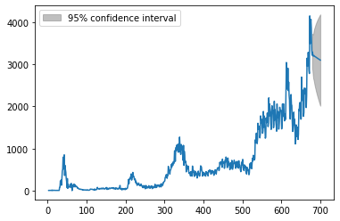
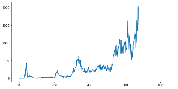
한국의 코로나 신규 확진자 예측해라(선형 시계열모델 + 비선형시계열 각각 한개씩 만들어라)
선형시계열 - arma 비선형 시계열 - arima
Show code cell content
ko = df[df.location =='South Korea'].reset_index(drop=True)
ko.head()
| location | date | total_cases | total_deaths | new_tests | population | new_vaccinations | ratio | new_cases | new_deaths | total_vacciantions | 7days_new_case | ratio_index | |
|---|---|---|---|---|---|---|---|---|---|---|---|---|---|
| 0 | South Korea | 2020-01-21 | 0.0 | 0.0 | 0.0 | 51305184.0 | 0.0 | 0.000000e+00 | 0.0 | 0.0 | 0.0 | 0.0 | 0.0 |
| 1 | South Korea | 2020-01-22 | 1.0 | 0.0 | 5.0 | 51305184.0 | 0.0 | 1.949121e-08 | 1.0 | 0.0 | 0.0 | 0.0 | 0.0 |
| 2 | South Korea | 2020-01-23 | 1.0 | 0.0 | 0.0 | 51305184.0 | 0.0 | 1.949121e-08 | 0.0 | 0.0 | 0.0 | 0.0 | 0.0 |
| 3 | South Korea | 2020-01-24 | 2.0 | 0.0 | 0.0 | 51305184.0 | 0.0 | 3.898242e-08 | 1.0 | 0.0 | 0.0 | 0.0 | 0.0 |
| 4 | South Korea | 2020-01-25 | 2.0 | 0.0 | 0.0 | 51305184.0 | 0.0 | 3.898242e-08 | 0.0 | 0.0 | 0.0 | 0.0 | 0.0 |
Show code cell content
# 선형모델 - arma.

from statsmodels.tsa.ar_model import AutoReg
mod = AutoReg(ko.new_cases, 3, old_names=False)
res = mod.fit()
print(res.summary())
fig = res.plot_predict(1,700)

# 비선형 모델 -arima 사용
from statsmodels.tsa.arima.model import ARIMA

model = ARIMA(ko.new_cases, order=(0,1,1))
model_fit = model.fit()
print(model_fit.summary())

forecast = model_fit.forecast(steps=24*7)

plt.figure(figsize=(10,5))
plt.plot(ko.new_cases)
plt.plot(forecast)
                            AutoReg Model Results
==============================================================================
Dep. Variable:              new_cases   No. Observations:                  679
Model:                     AutoReg(3)   Log Likelihood               -4376.552
Method:               Conditional MLE   S.D. of innovations            156.844
Date:                Sun, 04 Sep 2022   AIC                           8763.103
Time:                        19:54:21   BIC                           8785.684
Sample:                             3   HQIC                          8771.846
                                  679
================================================================================
                   coef    std err          z      P>|z|      [0.025      0.975]
--------------------------------------------------------------------------------
const           10.0652      7.966      1.264      0.206      -5.547      25.678
new_cases.L1     0.9978      0.037     27.163      0.000       0.926       1.070
new_cases.L2    -0.3117      0.052     -6.002      0.000      -0.413      -0.210
new_cases.L3     0.3080      0.038      8.196      0.000       0.234       0.382
                                    Roots
=============================================================================
                  Real          Imaginary           Modulus         Frequency
-----------------------------------------------------------------------------
AR.1            1.0045           -0.0000j            1.0045           -0.0000
AR.2            0.0037           -1.7978j            1.7978           -0.2497
AR.3            0.0037           +1.7978j            1.7978            0.2497
-----------------------------------------------------------------------------
                               SARIMAX Results
==============================================================================
Dep. Variable:              new_cases   No. Observations:                  679
Model:                 ARIMA(0, 1, 1)   Log Likelihood               -4422.919
Date:                Sun, 04 Sep 2022   AIC                           8849.837
Time:                        19:54:21   BIC                           8858.876
Sample:                             0   HQIC                          8853.336
                                - 679
Covariance Type:                  opg
==============================================================================
                 coef    std err          z      P>|z|      [0.025      0.975]
------------------------------------------------------------------------------
ma.L1          0.0072      0.025      0.286      0.775      -0.042       0.057
sigma2       2.73e+04    486.188     56.156      0.000    2.63e+04    2.83e+04
===================================================================================
Ljung-Box (L1) (Q):                   0.01   Jarque-Bera (JB):              8521.33
Prob(Q):                              0.94   Prob(JB):                         0.00
Heteroskedasticity (H):              21.35   Skew:                             2.60
Prob(H) (two-sided):                  0.00   Kurtosis:                        19.57
===================================================================================

Warnings:
[1] Covariance matrix calculated using the outer product of gradients (complex-step).
[<matplotlib.lines.Line2D at 0x7f7c43b44c70>]
Attention
3번
설문조사 데이터
데이터 출처 : 자체 제작
data Url : https://raw.githubusercontent.com/Datamanim/datarepo/main/adp/p3/problem3.csv
데이터 설명 : A ~ D까지의 그룹에게 각각 같은 설문조사를 하여 1-1,1-2,1-3…5-1,5-4 인 설문지를 푼 것이다.
문항은 영역별로 나뉘어 있고, 영역은 크게 5개이다(1~5)
각 영역의 세부문항은 4개씩 존재한다 (1-1,1-2,1-3,1-4 ~) 이 때 중간에 반대 문항이 들어가 있다.
예를 들어 1-1 문제가 “나는 시간약속을 잘 지킨다.”라는 문제라면 1-3의 문제는 “나는 시간약속을 잘 지키지 않는다.” 라는 역문제로 구성 되어있다.
각 영역의 3번문항의 1번문항의 역문제이다. 모든 답변은 5점 척도이다. 문제를 풀기전 모든 역문항의 경우 점수를 변환(6점을 빼서) 작업이 필요하다
import pandas as pd
df =pd.read_csv('https://raw.githubusercontent.com/Datamanim/datarepo/main/adp/17/problem3.csv')
df.head()
| userid | group | Q1-1 | Q1-2 | Q1-3 | Q1-4 | Q2-1 | Q2-2 | Q2-3 | Q2-4 | ... | Q3-3 | Q3-4 | Q4-1 | Q4-2 | Q4-3 | Q4-4 | Q5-1 | Q5-2 | Q5-3 | Q5-4 | |
|---|---|---|---|---|---|---|---|---|---|---|---|---|---|---|---|---|---|---|---|---|---|
| 0 | 0 | A | 5 | 2 | 1 | 2 | 4 | 5 | 3 | 3 | ... | 1 | 1 | 5 | 2 | 5 | 3 | 3 | 4 | 3 | 4 |
| 1 | 1 | A | 2 | 2 | 3 | 3 | 4 | 3 | 1 | 4 | ... | 2 | 3 | 4 | 3 | 5 | 3 | 1 | 2 | 1 | 1 |
| 2 | 2 | A | 1 | 3 | 4 | 4 | 2 | 1 | 4 | 4 | ... | 4 | 2 | 1 | 3 | 4 | 1 | 3 | 3 | 2 | 5 |
| 3 | 3 | A | 3 | 3 | 4 | 2 | 2 | 4 | 4 | 3 | ... | 2 | 3 | 3 | 4 | 2 | 4 | 1 | 1 | 3 | 2 |
| 4 | 4 | A | 3 | 1 | 2 | 3 | 4 | 3 | 4 | 1 | ... | 5 | 1 | 3 | 2 | 3 | 1 | 3 | 2 | 5 | 4 |
5 rows × 22 columns
3-1번
역문항을 변환 한 후 각 그룹(A~D)의 영역(Q1~Q5)별 응답의 평균, 표준편차, 왜도, 첨도를 구하라. (각 통계량 별로 4x5 dataframe 생성)
Show code cell content
# 역변환
for num in range(1,6):
    df[f'Q{num}-3'] =6 -df[f'Q{num}-3']

for num in range(1,6):
    col_lst = ['group']
    for col in range(1,5):
        col_lst.append(f'Q{num}-{col}')

    target = df[col_lst]

    targetdf =target.set_index('group').unstack().to_frame().reset_index()[['group',0]].rename(columns ={0: f'Q{num}'})

    display(targetdf.groupby('group').agg(['mean','std','skew',pd.DataFrame.kurt]))
| Q1 | ||||
|---|---|---|---|---|
| mean | std | skew | kurt | |
| group | ||||
| A | 3.016 | 1.263860 | -0.077803 | -1.087887 |
| B | 3.042 | 1.242489 | -0.126751 | -1.022905 |
| C | 3.030 | 1.243642 | -0.050626 | -1.033246 |
| D | 2.991 | 1.264325 | -0.069421 | -1.081406 |
| Q2 | ||||
|---|---|---|---|---|
| mean | std | skew | kurt | |
| group | ||||
| A | 3.058 | 1.236999 | -0.129390 | -0.997133 |
| B | 3.048 | 1.266215 | -0.111043 | -1.060834 |
| C | 3.063 | 1.256427 | -0.122030 | -1.046603 |
| D | 3.091 | 1.249913 | -0.166334 | -1.018150 |
| Q3 | ||||
|---|---|---|---|---|
| mean | std | skew | kurt | |
| group | ||||
| A | 2.992 | 1.268679 | -0.061600 | -1.098330 |
| B | 3.050 | 1.238965 | -0.117158 | -1.035672 |
| C | 3.023 | 1.248210 | -0.102330 | -0.988577 |
| D | 3.034 | 1.255556 | -0.128043 | -1.043094 |
| Q4 | ||||
|---|---|---|---|---|
| mean | std | skew | kurt | |
| group | ||||
| A | 3.043 | 1.255678 | -0.090314 | -1.028166 |
| B | 3.041 | 1.240507 | -0.071541 | -1.014676 |
| C | 3.014 | 1.283531 | -0.074531 | -1.100094 |
| D | 3.080 | 1.268546 | -0.144620 | -1.006126 |
| Q5 | ||||
|---|---|---|---|---|
| mean | std | skew | kurt | |
| group | ||||
| A | 3.088 | 1.256119 | -0.102638 | -1.053632 |
| B | 2.983 | 1.272136 | -0.055805 | -1.080934 |
| C | 2.987 | 1.260325 | -0.068696 | -1.071557 |
| D | 2.989 | 1.250777 | -0.065315 | -1.055332 |
3-2번
그룹별로 Q1-1문항의 차이가 존재하는지 anova분석을 시행하라
Show code cell content
from scipy.stats import shapiro
a = df[df.group =='A']['Q1-1']
b = df[df.group =='B']['Q1-1']
c = df[df.group =='C']['Q1-1']
d = df[df.group =='D']['Q1-1']

print('a p-value',shapiro(a)[1])
print('b p-value',shapiro(b)[1])
print('c p-value',shapiro(c)[1])
print('d p-value',shapiro(d)[1])


from scipy.stats import levene

# 등분산 만족한다
print(levene(a,b,c,d))
print()

# 정규성을 만족하지 않기 때문에 kruskal-wallis H test를 통해 분산 분석 진행
from scipy.stats import kruskal
kruskal(a,b,c,d)

# 4개의 그룹은 통계적으로 유의한 차이가 없다
a p-value 4.089666539447423e-12
b p-value 1.2895768654319628e-11
c p-value 1.4126045819184974e-11
d p-value 4.2081052184506085e-12
LeveneResult(statistic=0.24718103455049822, pvalue=0.8633690011210747)
KruskalResult(statistic=4.567127187870985, pvalue=0.20638028098088249)
3-3번
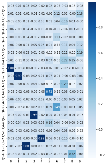
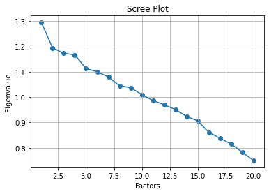
탐색적 요인분석을 수행하고 결과를 시각화 하라
Show code cell content
ana = df.drop(columns = ['userid','group'])
#실제 adp 패키지리스트에는 존재함
#!pip install factor-analyzer

from factor_analyzer.factor_analyzer import calculate_bartlett_sphericity
chi_square_value,p_value=calculate_bartlett_sphericity(ana)
chi_square_value, p_value

# 요인성 평가 결과 요인성 평가에 적합한 p-value( <0.05)를 확인

from factor_analyzer import FactorAnalyzer
from factor_analyzer.factor_analyzer import calculate_kmo
kmo_all,kmo_model=calculate_kmo(ana)
kmo_model
# kmo 결과 0.6 이하는 부적합하다 본다


fa = FactorAnalyzer(n_factors=25,rotation=None)
fa.fit(ana)
#Eigen값 체크
ev, v = fa.get_eigenvalues()
plt.scatter(range(1,ana.shape[1]+1),ev)
plt.plot(range(1,ana.shape[1]+1),ev)
plt.title('Scree Plot')
plt.xlabel('Factors')
plt.ylabel('Eigenvalue')
plt.grid()
plt.show()

#eigenvalue가 1이 되는지점인 10개의 요인이 선택에 적합한 숫자로 확인


fa = FactorAnalyzer(n_factors=10, rotation="varimax") #ml : 최대우도 방법
fa.fit(ana)
efa_result= pd.DataFrame(fa.loadings_, index=ana.columns)
plt.figure(figsize=(6,10))
sns.heatmap(efa_result, cmap="Blues", annot=True, fmt='.2f')
<AxesSubplot:>