작업형 제 1유형 예시문제¶

import pandas as pd
import matplotlib.pyplot as plt

df = pd.read_csv('https://raw.githubusercontent.com/Datamanim/dataq/main/mtcars.csv',index_col=0)

Question 1

mtcars 데이터셋(mtcars.csv)의 qsec 컬럼을 최소 최대 척도(min-max scale)로 변환한 후 0.5보다 큰 값을 가지는 레코드 수를 구하시오.

X = df['qsec']
X_MinMax = (X - X.min(axis=0)) / (X.max(axis=0) - X.min(axis=0))

overNum = len(X_MinMax[X_MinMax>0.5])

X_MinMax.values

array([0.23333333, 0.3       , 0.48928571, 0.58809524, 0.3       ,
       0.68095238, 0.15952381, 0.6547619 , 1.        , 0.45238095,
       0.52380952, 0.3452381 , 0.36904762, 0.41666667, 0.41428571,
       0.3952381 , 0.34761905, 0.59166667, 0.47857143, 0.64285714,
       0.65595238, 0.28214286, 0.33333333, 0.10833333, 0.30357143,
       0.52380952, 0.26190476, 0.28571429, 0.        , 0.11904762,
       0.01190476, 0.48809524])

overNum

Question 2

mtcars 데이터셋(mtcars.csv)의 qsec 컬럼을 표준정규분포 데이터 표준화 (standardization) 변환 후 최대, 최소값을 각각 구하시오.

mean = df.qsec.mean()
std = df.qsec.std()
scale = (df.qsec-mean)/std

Max = max(scale)
Min = min(scale)

print(Max,Min)

2.826754592962484 -1.8740102832334835

Question 3

*mtcars 데이터셋(mtcars.csv)의 wt 컬럼의 이상치(IQR 1.5 외부에 존재하는)값들을 outlier 변수에 저장하라

import numpy as np

q75,q50 ,q25 = np.percentile(df.wt, [75 ,50,25])
iqr = q75 - q25

outlier = df.wt[(df.wt>= q75 + iqr*1.5) | (df.wt <= q25 - iqr*1.5)].values

outlier

array([5.25 , 5.424, 5.345])

Question 4

mtcars 데이터셋에서 mpg변수와 나머지 변수들의 상관계수를 구하여 다음과 같이 내림차순 정렬하여 표현하라

corResult = df.corr()[['mpg']][1:].sort_values('mpg',ascending=False)

corResult

	mpg
drat	0.681172
vs	0.664039
am	0.599832
gear	0.480285
qsec	0.418684
carb	-0.550925
hp	-0.776168
disp	-0.847551
cyl	-0.852162
wt	-0.867659

Question 5

mtcars 데이터셋에서 mpg변수를 제외하고 데이터 정규화 (standardscaler) 과정을 진행한 이후 PCA를 통해 변수 축소를 하려한다. 누적설명 분산량이 92%를 넘기기 위해서는 몇개의 주성분을 선택해야하는지 설명하라

pcaDf = df.iloc[:,1:]
pcaDf = sc.fit_transform(pcaDf)

from sklearn.decomposition import PCA

componentsNum=10
pca = PCA(n_components=componentsNum) 
printcipalComponents = pca.fit_transform(pcaDf)
principalDf = pd.DataFrame(data=printcipalComponents, columns = ['component'+str(x) for x in range(componentsNum)])

componentDf = pd.DataFrame(pca.explained_variance_ratio_,columns=['cumsumVariance']).cumsum().reset_index()
componentDf['index'] +=1
componentDf=componentDf.rename(columns={'index':'componentsCount'})

componentDf

	componentsCount	cumsumVariance
0	1	0.576022
1	2	0.840986
2	3	0.900708
3	4	0.927658
4	5	0.949883
5	6	0.970895
6	7	0.984187
7	8	0.992255
8	9	0.997620
9	10	1.000000

Question 6

mtcars 의 index는 (업체명) - (모델명)으로 구성된다. (valiant는 업체명) mtcars에 ‘brand’ 컬럼을 추가하고 value 값으로 업체명을 입력하라

df['brand'] = pd.DataFrame(list(df.index.str.split(" ")))[0].values

df.head(5)

	mpg	cyl	disp	hp	drat	wt	qsec	vs	am	gear	carb	brand
Mazda RX4	21.0	6	160.0	110	3.90	2.620	16.46	0	1	4	4	Mazda
Mazda RX4 Wag	21.0	6	160.0	110	3.90	2.875	17.02	0	1	4	4	Mazda
Datsun 710	22.8	4	108.0	93	3.85	2.320	18.61	1	1	4	1	Datsun
Hornet 4 Drive	21.4	6	258.0	110	3.08	3.215	19.44	1	0	3	1	Hornet
Hornet Sportabout	18.7	8	360.0	175	3.15	3.440	17.02	0	0	3	2	Hornet

Question 7

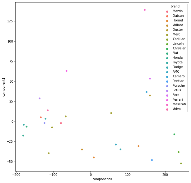
추가된 brand 컬럼을 제외한 모든 컬럼을 통해 pca를 실시한다. 2개의 주성분과 brand컬럼으로 구성된 새로운 데이터 프레임을 출력하고, brand에 따른 2개 주성분을 시각화하여라 (brand를 구분 할수 있도록 색이다른 scatterplot, legend를 표시한다)

from sklearn.decomposition import PCA

pcaDf = df.drop('brand',axis=1)

componentsNum=2
pca = PCA(n_components=componentsNum) 
printcipalComponents = pca.fit_transform(pcaDf)
principalDf = pd.DataFrame(data=printcipalComponents, columns = ['component'+str(x) for x in range(componentsNum)])

principalDf['brand'] = df['brand'].values

import seaborn as sns
plt.figure(figsize=(10,10))
sns.scatterplot(x='component0',y='component1',hue='brand',data=principalDf)

plt.show()

DataManim

작업형 제 1유형 예시문제

작업형 제 1유형 예시문제¶