다이아몬드 데이터셋¶

import pandas as pd
df = pd.read_csv('https://raw.githubusercontent.com/Datamanim/dataq/main/diamonds.csv',index_col=0)

Question 1

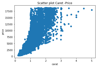
carat과 price의 경향을 비교하기 위한 scatterplot그래프를 출력하시오

import matplotlib.pyplot as plt

plt.scatter(df['carat'],df['price'])
plt.xlabel('carat')
plt.ylabel('price')
plt.title('Scatter plot Caret -Price')
plt.show()

Question 2

carat과 price사이의 상관계수와 상관계수의 p-value값은?

corr_by_pandas = df[['carat','price']].corr().iloc[0,1]

print(corr_by_pandas)

0.9215913011935697

from scipy import stats

corr_by_scipy ,pv= stats.pearsonr(df['carat'],df['price'])

print(corr_by_scipy)

0.9215913011934769

print(pv)

0.0

Question 3

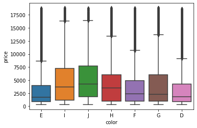
color에 따른 price 값의 분포는 아래와 같다.

import seaborn as sns

sns.boxplot(data=df,x='color',y='price')

<AxesSubplot:xlabel='color', ylabel='price'>

Question 3-1

Diamond의 평균가격은 3932로 알려져있다. ‘H’ color를 가지는 다이아몬드 집단의 평균에 대한 일표본 t검정을 시행하려한다. 통계량과 pvalue값을 구하시오. 유의수준 0.05에서 귀무가설 채택여부를 boolean 값으로 표현할 변수(hypo) 만들고 출력하시오

H_prop = df[df['color'] == 'H']
static, pv = stats.ttest_1samp(H_prop['price'], 3932)

if pv<0.05:
    hypo = False
else:
    hypo = True

print(static)
print(pv)
print(hypo)

11.988997411117696
7.569973305218302e-33
False

Question 3-2

그래프상에서 ‘F’와 ‘G’는 평균이 유사해보인다.이를 확인하기 위해 집단간 등분산(levene,fligner,bartlett) 검정을 시행 후 결과를 출력하고조건에 맞는 독립표본 t검정을 시행하라

F = df[df['color'] == 'F']
G = df[df['color'] == 'G']

leve = stats.levene(F['price'], G['price'])
fli = stats.fligner(F['price'], G['price'])
bartlet= stats.bartlett(F['price'], G['price'])

print(leve)
print(fli)
print(bartlet)

LeveneResult(statistic=53.627886257416655, pvalue=2.511093007074788e-13)
FlignerResult(statistic=37.04347553879807, pvalue=1.155244880009172e-09)
BartlettResult(statistic=47.52732212008511, pvalue=5.424264079418252e-12)

등분산 조건 확인시 귀무가설 기각(p-value <0.05), 유의수준하에 ‘F와 G 집단간 분산은 같지 않다’

t_test_FG =stats.ttest_ind(G['price'], F['price'], equal_var = False)

t_test_FG

Ttest_indResult(statistic=5.045279980436125, pvalue=4.5670321227041464e-07)

독립표본 t검정 시행시 귀무가설 기각(p-value <0.05), 유의수준하에 ‘F와 G 집단간 평균은 같지 않다’

Question 3-3

color ‘F’,’G’,’D’ 세집단의 price값들에 대해 anova분석을 시행하라.

등분산검정

D = df[df['color'] == 'D']

levene = stats.levene(F['price'], D['price'], G['price'])
fligner =stats.fligner(F['price'], D['price'], G['price'])
bartlett =stats.bartlett(F['price'], D['price'], G['price'])

print(bartlett)
print(fligner)
print(levene)

BartlettResult(statistic=289.14364432535103, pvalue=1.634012581050329e-63)
FlignerResult(statistic=494.64591695585733, pvalue=3.881538382653518e-108)
LeveneResult(statistic=118.97521469312785, pvalue=3.557425577381817e-52)

정규성검정

print(FG)
print(FD)
print(GD)

KstestResult(statistic=0.06151941343574685, pvalue=1.852300346010811e-17)
KstestResult(statistic=0.09505504118130681, pvalue=6.994405055138486e-15)
KstestResult(statistic=0.12093708375978551, pvalue=2.0167762615717943e-54)

anova = stats.f_oneway(F['price'], D['price'], G['price'])

anova

F_onewayResult(statistic=101.1811790316069, pvalue=1.6513790091285713e-44)

세집단의 분산분석 시행결과 귀무가설을 기각하고 (p-value <0.05) 유의수준 하에서 세집단 중 어느 두집단의 평균은 같지 않다(정확한 검정을 위해서는 사후검정실시해야함)

Question 4

연속형 변수(carat,depth,table,price,x,y,z) 각각의 이상치(1,3분위값에서 IQR*1.5 외의 값) 갯수를 데이터 프레임(변수명 ratio_df, 비율의 내림차순 정렬)으로 아래와 같이 나타내어라.

lst = []
for col in ['carat','depth','table','price','x','y','z']:
    target = df[col]
    iqr = target.quantile(0.75) - target.quantile(0.25)
    outlier = target.loc[(target > target.quantile(0.75) +iqr*1.5) | (target < target.quantile(0.25) - iqr*1.5)]
    lst.append([col,len(outlier)])
ratio_df = pd.DataFrame(lst).rename(columns={0:'column',1:'ratio'}).sort_values('ratio',ascending=False)

ratio_df

	column	ratio
3	price	3540
1	depth	2545
0	carat	1889
2	table	605
6	z	49
4	x	32
5	y	29

Question 5

color에 따른 price의 max, min, 평균값을 colorDf 변수에 저장하고 아래와 같이 출력하는 코드를 작성하라

colorDf = df.groupby(['color'])['price'].agg(['max','min','mean'])

colorDf

	max	min	mean
color
D	18693	357	3169.954096
E	18731	326	3076.752475
F	18791	342	3724.886397
G	18818	354	3999.135671
H	18803	337	4486.669196
I	18823	334	5091.874954
J	18710	335	5323.818020

Question 6

전체 데이터중 color의 발생빈도수에 따라 labelEncoding(빈도수 적은것 : 1, 빈도수 증가할수록 1씩증가)을 하고 colorLabel 컬럼에 저장하고 cut에 따른 colorLabel의 평균값을 구하여라

dic= {x: i+1 for i, x in enumerate(list(df.groupby('color').size().sort_values().index))}

df['colorLabel'] = df['color'].map(lambda x: dic[x])

df['colorLabel'].head(3)

  6
  6
  6
Name: colorLabel, dtype: int64

mean_cut = df.groupby('cut')[['colorLabel']].mean()

mean_cut

	colorLabel
cut
Fair	4.516770
Good	4.562780
Ideal	4.769152
Premium	4.644913
Very Good	4.654362

Question 7

price의 값에 따른 구간을 1000단위로 나누고 priceLabel 컬럼에 저장하라. 저장시 숫자 순으로 label하고(0~1000미만 : 0,1000이상~2000미만 :1 …) 최종적으로 구간별 갯수(변수명:labelCount)를 출력하라

df['priceLabel'] = df['price'].map(lambda x: x//1000)
labelCount = df[['priceLabel']].value_counts().to_frame().reset_index().rename(columns={0:'counts'})

labelCount

	priceLabel	counts
0	0	14499
1	1	9704
2	2	6131
3	4	4653
4	3	4226
5	5	3174
6	6	2278
7	7	1669
8	8	1307
9	9	1076
10	10	935
11	11	824
12	12	702
13	13	603
14	15	514
15	14	503
16	16	424
17	17	406
18	18	312

DataManim

다이아몬드 데이터셋

다이아몬드 데이터셋¶